« July 2007 | Main | September 2007 »

August 2007

August 26, 2007

Is Competition a New Risk Factor?

Clifford Asness, a Chicago Ph.D. as well as Managing and Founding Principle of AQR Capital Management, recently said that imitators are a new risk factor. Joe Nocera's August 18, 2007 New York Times article on quantitative investing reports his interviews:

In the view of several big-time quants I spoke to, their big mistake was in not realizing that their little corner of Wall Street had become so crowded with imitators — and that when others were forced to sell, they were going to get hurt. Now they are all trying to figure out how to factor that into their thinking for the future — Mr. Asness very much included. “We have a new risk factor in our world,” he said (bold inserted).

In case you are new here this is my 8th and final post in a current series on the competition for customers and capital among leading investment banks. In it I describe a model to factor competition into your thinking about pricing equities. Then I apply the model to Morgan Stanley (NYSE: MS) in a group containing three direct competitors: Goldman Sachs (NYSE: GS); Lehman Brothers (NYSE: LEH) and Merrill Lynch (NYSE: MER). For background and details see my book Competing for Customers and Capital.

FACTORING IN COMPETITION
As you might expect, adding competition to a stock pricing model truly complicates the problem. Normally one would discount the projected future cash flow of a company. This approach won't do if you want to factor in the impact of competition. Put simply, competitors must be introduced in the very first step in the analysis and permitted to change the outcome in every other step through to the simultaneous pricing of their securities. This chart outlines my approach to factoring in competition.

Competitive_valuation_graphic_revis

1. The first step to factoring in competition is placing each company in a strategic group with others that share one or more customer segments and have access to similar resources. This makes it reasonable to pool their revenues.

2. The next is to determine the degree to which management has maximized earnings within that group. Managers that maximize earnings achieve the greatest possible productivity using the resources they have. Companies that fall short of this goal suffer from lower relative earnings productivity. As the short-fall grows, investors become more likely to notice and discount the company's stock. As Al Rappaport said in his classic book Creating Shareholder Value:

It is … productivity that the stock market reacts to when pricing a company’s shares.  Embedded in all shares is an implied long-term forecast about a company’s productivity – that is, its ability to create value in excess of the cost of producing it.  When the stock market prices a company’s shares according to a belief that the company will be able to create value over the long term, it is attributing [this belief] to the company’s long-term productivity or, equivalently, a sustainable competitive advantage.  In this way, productivity is the hinge on which both competitive advantage and shareholder value hang (Rappaport 1998, 69).

For a discussion of maximum earnings market share see my post "Double Bull's Eye for Morgan Stanley."

3. Calculate maximum earnings after enterprise marketing expenses. These expenses are reviewed in my post "Citigroup's Enterprise Marketing Expenses: The Middle Line."

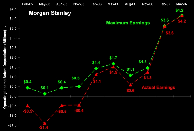
The difference between maximum and actual earnings is relative earnings productivity [REP]. The next chart documents Morgan Stanley's relative earnings productivity over the last ten quarters. After John Mack took the controls, the company marched steadily toward maximum earnings. By May, 2007 actual and maximum earnings were equal.

8_ms_rep_q105_q207_p01_2

4. Next, quantify the interaction between a firm's performance in the product markets and stock market in which it operates. The value-sales differential is the basis of this calculation. For details see my Marketing Science Institute paper "Marketing's Impact on Firm Value: The Value-Sales Differential."

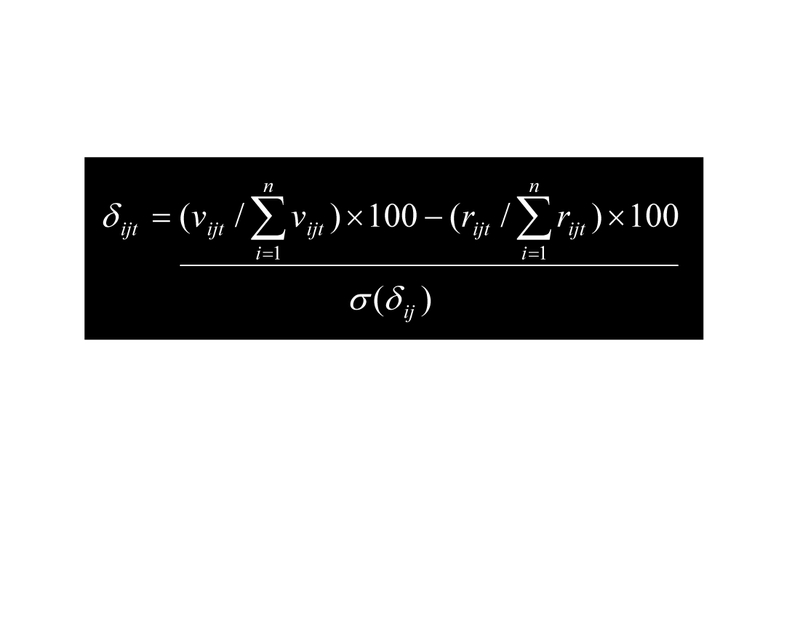
Value-sales differentials are adjusted for risk with a simple variation on the concept of risk-adjusted returns.  First, subtract a company's share of revenues in product markets from its share of market value in a security market. Second, divide each of these differentials by their standard deviation. The result is a risk-adjusted differential, RAD or delta (i,j,t) in this equation:

Delta_expanded_equation_p01_2

The first term on the right-hand side is the share of value [SOV] created by firm i, in strategic group j, in time period t. The second term is the share of revenues [SOR] generated by the firm. The denominator, sigma, is the standard deviation in a time series of firm differentials. In my post on "Citigroup's Differentials: 3D Marketing Metrics" I applied the risk-adjusted differential to a strategic group of investment banks. Delta, or RAD, is a standard normal variable (with mean zero and standard deviation of one). Dropping the subscripts and summations above the equation becomes:

Rad_reduced_equation_p01_4

Since I assume that management maximizes earnings I add a “hat” to the SOR term and solve for SOV.  The result is:

Sov_equation_p01

Think for a moment about the terms on the right-hand side of this equation.  The first term is the firm's most recent risk-adjusted differential. This is multiplied by its enterprise marketing risk and added to maximum earning’s market share. Not only simple, it makes sense.  When a company’s marketing risk is zero, the arithmetic product of RAD and Risk is zero.  In this event share of value equals share of revenue. Of course, I must assume that maximum earnings market share is independent of the company's enterprise marketing risk. In my experience with over 100 applications of the model, this assumption holds.

The next chart displays a plot of all possible shares of value at different levels of enterprise marketing risk and risk-adjusted differentials, for a maximum earnings market share of 34%.  As this surface map shows, when RAD equals zero share of value equals share of revenue over all levels of risk.

3d_surface_map_mems_34_p01

When enterprise marketing risk increases, for a given maximum earnings market share, the company's share of value deviates more from share of revenue.   And, as risk-adjusted differentials become more (or less) than zero, share of value again varies more (or less) from share of revenue.  At the lowest level of risk in this chart (0.5), share of value ranges from a low of 30% at a RAD of -8 to a high of 38% with a RAD of +8.%.  At the highest level of enterprise marketing risk in this chart (9.5), share of value ranges from 0% to 100%.  For unit changes in risk-adjusted differentials, share of value increases (decreases) by the level of risk.  For example, when risk is 5.0, share of value ranges from 0% to 74%.  It does so in increments of 5 for every one unit change in risk-adjusted differentials.

5. Given an estimate of strategic group market value, this last equation converts share of value into stock price:

Rad_reduced_equation_p01_3

A firm's stock price equals its shave of value times the strategic group's market value divided by the number of shares outstanding.

PREDICTING MORGAN STANLEY STOCK PRICE
What will happen to Morgan Stanley's stock price the day after the release of its 3rd quarter report at the end of September, 2007? By way of illustration, the following table predicts its price using the competitive stock valuation model described above.

Ms_price_q_ending_83107_p01

The company's enterprise marketing risk over the last ten quarters was 0.97. This is an extremely low risk. Which is why the stock price at either end of the 95% confidence interval does not vary much from the expected value. Morgan Stanley is in the tail of the risk distribution. The average enterprise marketing risk in my MSI study of 337 companies in 29 industries over ten years was 6.6.

Since I assume that management will, in fact, maximize earnings in the 3rd quarter with a 34% share of group revenues, only two questions remain. 

First, what will be Morgan Stanley's risk-adjusted differential? It was -0.31 at the end of the second quarter, up from -1.65 in the 3rd quarter of 2006. I take this most recent observation as the best estimate of its expected value. Since RADs have a standard deviation of one, we can set lower (in red) and upper (in green) 95% confidence interval estimates around this expected value.

Second, what will be the market value of the group of four investment banks? In the current volatile market environment the best estimate is the group's value on Friday ($238.4 billion), since all the information up to that time already was factored into prices.  From here on the rest is straight forward. I predict a low of price $72 and a high price of $81.

Morgan Stanley shares closed on Friday August 24, 2007 at $64.54 a share, giving it a market cap of $67.820 billion. The company's share of the group's value was 28.5%. If management maximizes earnings in the 3rd quarter, as it did in the 2nd, my model predicts investors will reward the company with a 33.7% share of the group's market value. The difference would amount to $12.5 billion or about an 18% premium over its closing value last Friday.

SOME FINAL THOUGHTS
Factoring in the effects of competition truly complicates the process of pricing securities. And certainly, my approach cannot be adapted to the performance of hedge funds without a lot of custom tailoring. But my hope is that it does suggest a way forward or at least food for thought about whether competition is indeed a new risk factor in Morgan Stanley's world, and yours.

A good friend of mine happens to be a financial economist. One day, a few years ago, while I was in the middle of writing my book I asked him what he thought about the working title: Competing for Customers and Capital. He said:

I know what you mean about the competition for customers, but I don't understand what you mean by the competition for capital. Capital markets are efficient; they're not imperfect like product markets.

What do you think? 

Thanks for visiting.

~V

August 19, 2007

Profit From the Dog Days of Summer

In late September Morgan Stanley (NYSE: MS) will file its report for the quarter ending August 31, 2007. This period coincides perfectly with the dog days of summer in the investment banking business.

The company's 3rd quarter report should display all the volatility in the financial markets during that period. What will it say about the company's performance under such pressure? And what effect will investor reactions have on Morgan Stanley's stock price? For a discussion of the theory behind this analysis see my book Competing for Customers and Capital.

This is 7th in my series of posts on the competition for customers and capital among four leading investment banks. In this post I speculate, using the tools enterprise marketing, on how Morgan Stanley management might profit from the dog days and its attendant market volatility. The other players in this analysis are Goldman Sachs (NYSE: GS), Lehman Brothers (NYSE: LEH) and Merrill Lynch (NYSE: MER).

HIGHLY SEASONAL REVENUES
The last ten quarters reveal a marked seasonality in the pattern of combined net revenues for these four investment banks. This chart shows the quarterly peaks and valleys over the period from February, 2005 through May, 2007 (white triangles).

Ib_revenues_p01

The historical dog days of summer are the valleys: $22 billion in August, 2005 and $25 billion in August 2006. The chart also includes a forecast (in blue) of the group's net revenue in August, 2007 if the 5.7% historical pattern of year-on quarterly CAGR holds true. In about six weeks we will know.

WHEN LESS IS MORE
Across a broad range of industries and companies, enterprise marketing expenses and revenues move in lock step. For example, in a study I did on the relationship between expenses and revenues of 497 companies in 30 industries in 2003 the correlation coefficent averaged 0.96, with a standard deviation of 0.07.

A similar relationship between enterprise marketing and net revenues appears for three of the four investment banks in this analysis. The correlation coefficients for GS, LEH and MER in the last ten quarters are 0.84, 1.00, and 0.64 respectively. But, MS was a different story: its correlation coefficient was -0.32. That's not a typo. The correlation was negative! Less was more for Morgan Stanley.

How did they do that? Management slashed the company's cost per dollar of net revenues from $1.23 in May, 2005 to $0.64 in May, 2007. In short, the company went from being very inefficient and losing $0.23 on every dollar of net revenue, to being highly efficient and earning $0.36 on every dollar.

For details on the enterprise marketing expenses of investment banks and their cost per dollar of revenue see my post "Citigroup Enterprise Marketing Expenses: The Middle Line."

THEORY MEETS REALITY
Market share attraction theory says that an efficient company will attract revenues in direct proportion to its share of enterprise marketing expenses, other things being equal. This chart shows Morgan Stanley's market share attraction from February, 2005 through May 2007. The vertical (green) axis is the company's share of net revenues in each of the ten quarters. The horizontal (red) axis is its share of enterprise marketing expenses in the same ten quarters.

Ms_attraction_p01

If Morgan Stanley had attracted customers in direct proportion to its share of enterprise marketing expenses, the relationship between share of revenue and share of expenses would be described by the dotted diagonal line in this chart.  In May, 2005 the company spent 43% of enterprise marketing resources to generate just 32% of revenues. After a long but steady march toward high enterprise marketing efficiency, in May, 2007 management spent 31% of the resources and generated 31% of the revenues. Clearly, management was not blindly setting expenses as a percent of revenues. Rather, it took a bee-line to that level of expenses the theory would predict. In May, 2007 its theoretical marketing efficiency ratio was exactly one, corresponding with that $0.64 per dollar of revenue.

A DOG DAY SCENARIO
Will the dog days be amplified by the down market? If so, how will the other players respond? What will Morgan Stanley management do while experiencing the down market during the 3rd quarter? How will they expect the competition to react under the same circumstances? Here's one of many possible scenarios that might play out:

1. Group revenues fall 12% from the dog day low.
2. Competitors cut enterprise marketing 15%.
3. Morgan Stanley hits 33.7% maximum earnings share.
4. Management drives cost per dollar down to $0.59.

CAPITALIZING ON THE DOG DAYS
This table compares Morgan Stanley's actual results in August, 2006 with forecast results in August, 2007, based on my scenario. I don't expect the forecast numbers to appear in their income statement when it's filed in late September. The purpose is not to crystal ball gaze. Rather it is to hypothesize on reasonable objectives that management might have set for the quarter, based on history and the principles of enterprise marketing.

Ms_actual_v_forecast_p01

These are challenging objectives. By achieving maximum earnings market share at 33.7%, net revenues would hold constant at $8.0 billion -- even in this double-down market. Further decreases in Morgan Stanley's cost per dollar of net revenue would hammer enterprise marketing expenses down from $7.4 billion in August, 2006 to $4.7 billion in August, 2007. The combination of these actions would drive operating income before depreciation up from $0.6 billion in the previous year to $3.3 billion in August, 2007. This pumps the ratio of earnings to net revenues up from 7% to 41%.

MORGAN STANLEY'S STOCK PRICE?
This is a pop quiz! If management actually delivered this performance in its 3rd quarter report, what would be its stock price on September 28? Here's a benchmark to consider: MS closed at $62.23 on Friday August 17, down from $85.82 on May 31, 2007. What do you think?

Thanks for visiting.

~V

August 12, 2007

The Faulty Ivory Towers

This is the 6th post in my series on the competition for customers and capital among leading investment banks. The players are Goldman Sachs (NYSE: GS), Lehman Brothers (NYSE: LEH), Merrill Lynch (NYSE: MER) and Morgan Stanley (NYSE: MS). In it I discover why investors believe net income is the top line for investment banks.

THE FOUR FACTORS MODEL RECONSIDERED
In the post on "Morgan Stanley, Merrill Lynch and the Fable of Three Bears" I defined the variables in my four factors model: competitors' enterprise marketing expenses [f], strategic group revenues [R], company percent gross margin [g dot] and company enterprise marketing efficiency [x]. Maximum earnings market share, symbolized in this chart as "m hat," is a non-linear function of these variables. You will find a proof of this model in my book, Competing for Customers and Capital (pages 251-52).

Mems_equation_p01

In most businesses, it happens that revenues and gross margins are pretty clearly defined. Take supermarkets for example. Revenues are the value of goods sold less returns and allowances. The percent gross margin is the ratio of revenues less the cost of these goods divided by revenues.  I believed the same revenue-margin model should be applied to investment banks by viewing revenues as the value of all services sold plus interest income. Interest expenses then become the "cost of goods sold" and gross margin is calculated just as it is in supermarkets. Following this approach Goldman Sachs gross revenues were $20.4 billion in May, 2007, interest expenses were $10.2 billion, so its gross margin was 50%. In case you want to calculate Goldman's maximum earnings market share, here are the other three inputs to the four factors model: f = $17.3 billion, R = $85.1 billion and x = 1.17.

WHY THE INTERMEDIATION APPROACH?
From the first post in this series on "Citigroup's Enterprise Marketing Expenses: The Middle Line" I adopted the intermediation approach to bank operations.

Manufacturing companies can easily load overhead expenses into the cost of good sold without anyone noticing. From an intermediation perspective the "cost of goods sold" in banking is interest expense. And banks aren't allowed to load overhead into interest expenses.

I was advised in a comment that "this is not the way practitioners see banking operations."  And in a later comment that, my analysis "will be most convincing to the practitioners if presented with the vocabulary familiar to the practitioners." But I remained convinced that the intermediation approach was the only way to go. In my post on "Double Bull's eye for Morgan Stanley" I attempted to shut out the "net income" approach with a quote from the Journal of Money, Credit and Banking. Why was I so committed to intermediation?

If banks actually had a zero cost of goods sold, like electronic futures exchange markets, my analysis would work just fine. But since interest expenses are a significant cost of doing business, ignoring them would cause distortions in a company's enterprise marketing efficiency and hence its maximum earnings market share.

This is true, but there's a larger issue. If all practitioners (both managers and investors) believe net income is an investment bank's top line, my theoretical distortions become their reality.

WHEN DISTORTION IS REALITY
Over the last week I began to apply my competitive stock valuation model to these four investment banks in preparation for a future post in this series. I've applied the model to over a hundred companies and it usually produces reasonable results. But the results for these banks weren't reasonable. I checked all the inputs and still the results didn't make sense. Predicted stock prices in May, 2008 were not consistent with closing prices in May, 2007. So I ran the numbers on net income and found a huge effect influencing investor perceptions. This table tells the story for Goldman Sachs.

Gs_intermediation_vs_net_income_q20

Using the net income approach (green), group revenues fall 56% from $85.1 to $37.1 billion. But practitioners don't (yet) look at group revenues in making investment decision, so this doesn't matter. Though Goldman's net revenues drop 50%, this is the way practitioners see banking operations. Gross margin is now 100% so gross profits remain unchanged at $10.2 billion. Enterprise marketing expenses and operating income before depreciation also are unchanged. But using the net income approach has a huge effect on an important bottom line ratio: earnings to revenues are less than half (4.5%) in the intermediation approach compared with the net income approach (10.3%). In short, what amounts to distortion in theory is reality in practice.

THE FAULTY IVORY TOWERS
So I've been trying to figure out why practitioners use net income, even though interest expenses are so important. Well, with all the focus on interest rates these days I finally saw the light. Interest expenses can't be treated as cost of goods sold because management has no control over the fed funds rate!

I should have listened to my reviewer's comments. Instead I succumbed to a weakness that inhabits the ivory towers ... the reluctance to give up a cherished approach to any problem. Needless to say, in my next post I'll use income net of interest.

What do you think?

~V

August 05, 2007

The Fable of the Three Bulls

This is the 5th post in my series on the competition for customers and capital among leading U.S. investment banks. The four banks in this strategic group are Goldman Sachs (NYSE: GS), Lehman Brothers (NYSE: LEH), Merrill Lynch (NYSE: MER) and Morgan Stanley (NYSE: MS). What follows is a time-series analysis of their search for market shares that maximize earnings after enterprise marketing expenses.

FOUR FACTORS MODEL AT A GLANCE
The concept of maximum earnings market share is straight out of microeconomics 101. You start by expressing your company's earnings after enterprise marketing expenses as a function of its market share in a strategic group. Then you take the first derivative of this function and solve for that market share where the difference between marginal costs and marginal earnings is zero. That's maximum earnings market share, symbolized in this chart as "m hat." You will find a proof of the four factors model in my book Competing for Customers and Capital (pages 251-52). [Click on the images to enlarge]

Mems_equation_p01

Two of these factors (in yellow) are outside your control: competitors' enterprise marketing expenses (f) and strategic group revenues (R). Happily, the two factors in green are under your control: your percent gross margins (g dot) and enterprise marketing efficiency (x).  When competing for customers, gross margin and marketing efficiency rule.

If you want to follow the logic through a detailed application to Southwest Airlines see my 14 minute Adobe Connect presentation on "The rule of Maximum Earnings." To check the results of applying the four factors model to Morgan Stanley in a single period see my last post in this series: "Double Bull's Eye for Morgan Stanley."

MORGAN STANLEY'S MAXIMUM EARNINGS MARKET SHARE
Management's climb to maximum earnings market share was slow, but sure. In this chart you will see that Morgan Stanley hit bottom on May 31, 2005 when its actual share of gross revenues (blue) exceeded its maximum earnings share (green) by 23.3 points. In that quarter MS posted a -$1.4 billion loss. Two weeks later, on June 13, embattled CEO Philip J. Purcell announced his retirement from Morgan Stanley. On June 30, 2005 John Mack was once again named the Chairman and CEO.

1_ms_mems_q105_q207_p01

By February, 2007 Morgan Stanley's management team had brought maximum earnings market share up to 32.4%, just 60 basis points above its actual market share of 31.8%. They undershot a bit more in the next quarter. This was a remarkable achievement. All the more so because the company's margins as a percent of gross revenues shrank from 60.0% in February 2005, to 41.6% in May 2007 -- as a result of sharply increased interest expenses.

How did MS management pull this off? It's simple in theory – they held the marginal cost of enterprise marketing constant while increasing marginal earnings. But in practice it was difficult. They had to cut enterprise marketing costs per dollar of revenue by 58% and simultaneously increase gross revenue by 139%. This chart tells the story of the impact these actions had on marginal costs and earnings.

2_ms_marginals_q105_q207_p01

Morgan Stanley's marginal cost (red) remained flat over this time at around $3.4 million per basis point. That's the enterprise marketing cost of the last 1/100th of a point at a 31.71% share of gross revenues. The company's marginal earnings per basis point (green) steadily increased. Looking back at May, 2005 the last one-hundredth of a share point returned just $1.9 million in operating income before depreciation. The company lost $1.5 million on that enterprise marketing transaction. Then management initiated an upward trend that continued through February, 2007 when the difference between marginal cost and earnings per basis point was about $100K.

MORGAN STANLEY'S MARCH TO MAXIMUM EARNINGS
Here's a more dramatic portrayal of Morgan Stanley's march to maximum earnings over the 10 quarters ended May, 2007.

3_ms_earnings_q105_q207_p01

Maximum potential earnings (green) ranged from a low of $0.1 billion in May, 2005 to a high of $4.2 billion in May, 2007. By then, maximum and actual earnings (red) were effectively equal. Looks like John Mack really knows how to run an investment bank.

MORGAN STANLEY'S ENTERPRISE MARKETING EXPENSES
How far out of line were Morgan Stanley's enterprise marketing expenses when Mr. Mack took the controls? This chart compares the actual with the theoretical enterprise marketing expenses required to maximize operating income before depreciation.

4_ms_expenses_q105_q207_p01

Actual expenses (red) remained flat at around $7.35 billion in every quarter. In May, 2005 MS would have spent $1.5 billion (green) on enterprise marketing if it had maximized earnings.  The company actually spent $7.4 billion. The gap between actual and maximum earnings expenses (green) was nearly $6 billion. Two years later the gap had narrowed to $200 million – in under-spending on enterprise marketing resources!

As I reported in "Reconsidering Citigroup: The Middle Line and 3D Marketing," Morgan Stanley management drove the company's enterprise marketing costs per dollar (CPD) of gross revenue down from $0.63 to $0.26 over the ten quarters. In the process their normalized enterprise marketing efficiency ratio improved from 1.54 to 0.93.  By May, 2007 MS paid just 93 cents for resources that cost an average competitor $1.00. Since this normalized efficiency ratio is a theoretical construct that cannot be observed, it cannot be managed. But the CPD can be. Still the two are highly correlated; in this case the correlation was +0.90.

MERRILL LYNCH'S SEARCH FOR MAXIMUM EARNINGS
Was John Mack just lucky? He took Morgan Stanley over at the right time. The Bull market was hitting its stride. But if he was just lucky, why did Merrill Lynch's search for maximum earnings miss the mark so far?

5_mer_mems_q404_q107_p01

In this chart Merrill Lynch looks like the golfer searching for a ball lost deep in the rough. Only in one quarter did management come close to maximum earnings market share. Operating in the same period, with similar resources, MER missed the mark in August, 2005 by -19.4 share points and -$1.0 billion in earnings. And again in August, 2006 by -21.5 share points and -$1.4 billion in earnings. That is to say, Merrill Lynch spent way too much on enterprise marketing resources; its maximum earnings market share was far less than its actual share in 8 of the 10 quarters.

Unlike Morgan Stanley, Merrill Lynch made an uncertain approach to maximum earnings. As the next chart shows, the company oscillated between quarters of relatively small differences between actual and maximum earnings and quarters of large gaps. For example a $900 million earnings shortfall in August, 2005 was followed by a $1.4 billion shortfall in August 2006 and another $900 million shortfall in the next quarter. In the last two quarters, Merrill Lynch management closed in on the sweet spot. Investors don't like that kind of volatility.

6_mer_earnings_q404_q107_p01

Neither Goldman Sachs nor Lehman Brothers came anywhere near this close to maximizing earnings. Over the 10 quarters both GS and LEH systematically and significantly under-spent on enterprise marketing resources. How can a company under-spend on enterprise marketing? Try this fable on for size.

THE FABLE OF THE THREE BULLS
Once upon a time three baby bulls lived in a pasture with their mother. Whenever it was time to be nursed the first baby bull would say: "Mama, I want the most milk so I can grow up to be the strongest of all." She would reply: "Yes, dear." Then the second baby bull would say: "Mama, I want the least milk so I can grow up to be the most nimble of all." She would reply: "Yes, dear." The third baby bull would say: "Mama I want just the right amount of milk so I can be both strong and nimble." She would say: "How much is that, dear?"

What's the moral of this story? Spend just enough to maximize earnings and your firm will be both strong and nimble. What do you think?

~V